Notes on Diffusion Models and Flow Matching

Entropy and KL Divergence

Self-information

For an event of probability \(p\), its self-information is

\[ I = -\log p = \log \frac{1}{p} \]

which is also the optimal code length (e.g. Huffman) assigned to that event. Rare events (small \(p\)) need more bits to encode.

Entropy and cross entropy

Let \(p\) be the true distribution and \(q\) a model of it. Coding samples from \(p\) gives an average code length of

\[ \begin{aligned} \text{Entropy:} \quad & H(p) = \mathbb{E}_{p}[-\log p] = -\int p(x)\log p(x)\,\mathrm{d}x \\[4pt] \text{Cross entropy:} \quad & H(p, q) = \mathbb{E}_{p}[-\log q] = -\int p(x)\log q(x)\,\mathrm{d}x \end{aligned} \]

using the optimal code for \(p\) and the (mismatched) optimal code for \(q\) respectively. A mismatched code is never shorter, so \(H(p,q) \ge H(p)\).

KL divergence

The extra code length caused by the mismatch is the KL divergence:

\[ D_{\text{KL}}(p \parallel q) = H(p,q) - H(p) = \mathbb{E}_{p}\left[\log \frac{p}{q}\right] \]

with \(D_{\text{KL}} \ge 0\), and \(D_{\text{KL}}(p \parallel q) \ne D_{\text{KL}}(q \parallel p)\).

How to memorize KL divergence

Stand in the true world and measure the true/fake ratio: in \(D_{\text{KL}}(\textbf{True} \parallel \textbf{Fake})\) the left argument is the one we take the expectation over, and inside the log truth sits on the numerator.

Varitional Autoencoders (VAEs)

Evidence Lower Bound (ELBO)

Model the observation \(x\) jointly with a latent variable \(z\). The likelihood can be recovered from \(p(x,z)\) in two ways:

\[ p(x) = \int p(x,z)\,\mathrm{d}z, \qquad p(x) = \frac{p(x,z)}{p(z \mid x)} \]

Both are intractable: the first integrates over all latents, the second requires the true posterior \(p(z\mid x)\). Instead we introduce a variational distribution \(q_\phi(z \mid x)\) approximating \(p(z\mid x)\), and maximise the evidence lower bound

\[ \log p(x) \ge \mathbb{E}_{q_\phi(z\mid x)}\left[\log \frac{p(x,z)}{q_\phi(z\mid x)}\right] \]

Prior, likelihood, evidence, posterior

Prior \(p(z)\) — belief about the latent before seeing any data; in VAEs fixed to \(\mathcal{N}(0, I)\).
Conditional likelihood \(p_\theta(x \mid z)\) — how well a given latent reconstructs the data; the decoder.
Marginal likelihood (evidence) \(p(x) = \int p(x\mid z)p(z)\,\mathrm{d}z\) — total probability the model assigns to the observed data, with the latent integrated out.
Posterior \(p(z \mid x)\) — latent (prior) inferred from the data. Intractable, approximated by the encoder \(q_\phi(z\mid x)\).

In one sentence: the encoder infers the posterior over \(z\), the decoder maximises the likelihood of \(x\) given \(z\), and the prior keeps the latent space from drifting arbitrarily.

Derivation 1 (Jensen). From the marginalisation form,

\[ \begin{aligned} \log p(x) &= \log \int p(x,z)\frac{q_\phi(z\mid x)}{q_\phi(z\mid x)}\,\mathrm{d}z \\[4pt] &= \log \mathbb{E}_{q_\phi(z\mid x)}\left[\frac{p(x,z)}{q_\phi(z\mid x)}\right] \ge \mathbb{E}_{q_\phi(z\mid x)}\left[\log \frac{p(x,z)}{q_\phi(z\mid x)}\right] \end{aligned} \]

This gives the bound but hides why the gap exists.

How to memorize the Jensen's inequality

For a concave \(f\) (such as \(\log\)), \(\mathbb{E}[f(X)] \le f(\mathbb{E}[X])\): averaging first, then taking the log, is larger.

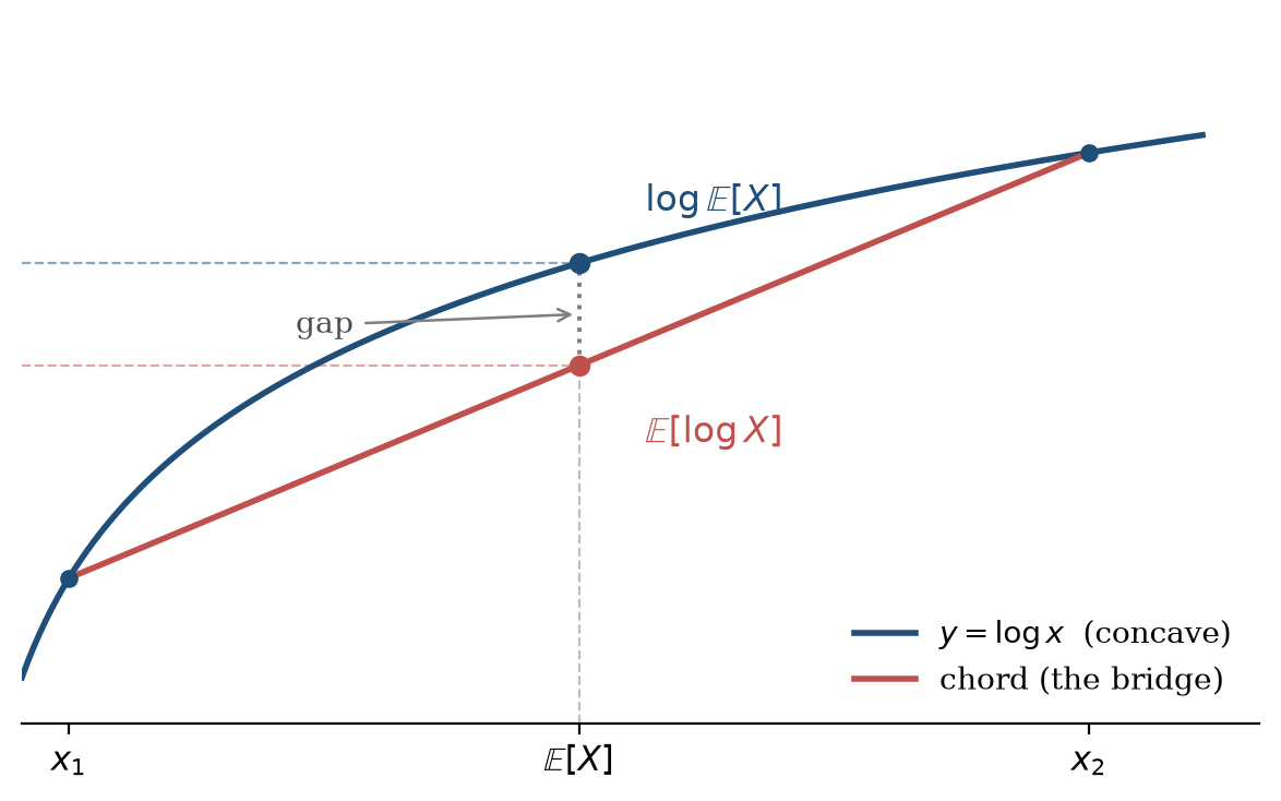
Jensen's inequality for the concave log

Derivation 2 (explicit gap). The key trick is that \(\log p(x)\) does not depend on \(z\), so it is a constant with respect to \(q_\phi(z\mid x)\) and can be pushed inside an expectation for free:

\[ \log p(x) = \log p(x) \cdot \underbrace{\int q_\phi(z\mid x)\,\mathrm{d}z}_{=\,1} = \int q_\phi(z\mid x)\log p(x)\,\mathrm{d}z = \mathbb{E}_{q_\phi(z\mid x)}\big[\log p(x)\big] \]

Starting from there and applying the chain-rule form \(p(x) = p(x,z)/p(z\mid x)\),

\[ \begin{aligned} \log p(x) &= \mathbb{E}_{q_\phi(z\mid x)}\big[\log p(x)\big] && \text{(constant in } z\text{)} \\[4pt] &= \mathbb{E}_{q_\phi(z\mid x)}\left[\log \frac{p(x,z)}{p(z\mid x)}\right] && \text{(chain rule)} \\[4pt] &= \mathbb{E}_{q_\phi(z\mid x)}\left[\log \frac{p(x,z)\,q_\phi(z\mid x)}{p(z\mid x)\,q_\phi(z\mid x)}\right] && \text{(multiply by } 1 = q_\phi/q_\phi) \\[4pt] &= \mathbb{E}_{q_\phi(z\mid x)}\left[\log \frac{p(x,z)}{q_\phi(z\mid x)}\right] + \mathbb{E}_{q_\phi(z\mid x)}\left[\log \frac{q_\phi(z\mid x)}{p(z\mid x)}\right] && \text{(split the expectation)} \\[4pt] &= \underbrace{\mathbb{E}_{q_\phi(z\mid x)}\left[\log \frac{p(x,z)}{q_\phi(z\mid x)}\right]}_{\text{ELBO}} + \underbrace{D_{\text{KL}}\big(q_\phi(z\mid x) \parallel p(z\mid x)\big)}_{\ge\, 0} && \text{(definition of KL)} \end{aligned} \]

So the evidence equals the ELBO plus the KL between the approximate and true posterior — the term Jensen's inequality silently discarded. Two consequences:

The bound holds because the gap is a non-negative KL.
Maximising the ELBO is exactly equivalent to minimising KL of posterior: \(D_{\text{KL}}(q_\phi(z\mid x) \parallel p(z\mid x))\), which we cannot minimise directly since \(p(z\mid x)\) is unknown.\(\log p(x)\) is constant in \(\phi\), so

Encoder–decoder form. Expanding \(p(x,z) = p_\theta(x\mid z)p(z)\) splits the ELBO into

\[ \mathbb{E}_{q_\phi(z\mid x)}\left[\log \frac{p(x,z)}{q_\phi(z\mid x)}\right] = \underbrace{\mathbb{E}_{q_\phi(z\mid x)}\left[\log p_\theta(x\mid z)\right]}_{\text{reconstruction}} - \underbrace{D_{\text{KL}}\big(q_\phi(z\mid x) \parallel p(z)\big)}_{\text{prior matching}} \]

where \(q_\phi(z\mid x)\) is the encoder and \(p_\theta(x\mid z)\) the decoder.

Variational Autoencoders

A VAE directly maximises the ELBO jointly over \(\phi\) (encoder) and \(\theta\) (decoder).

The reconstruction term forces the latents to retain enough information to regenerate \(x\).
The prior matching term keeps \(q_\phi(z\mid x)\) close to \(p(z)\), preventing the encoder from collapsing into a Dirac delta.

Why variational?

The name refers to optimising over a family of distributions: we search for the best \(q_\phi(z\mid x)\) amongst all posteriors parameterised by \(\phi\). Since \(\log p(x)\) is constant in \(\phi\), maximising the ELBO is equivalent to minimising the KL divergence between the approximate and true posterior:

\[ \max_\phi \ \text{ELBO} \iff \min_\phi \ D_{\text{KL}}\big(q_\phi(z\mid x) \parallel p(z\mid x)\big) \]

Parameterisation. The encoder \(\phi\) is taken to be a diagonal Gaussian and the prior a standard Gaussian:

\[ q_\phi(z\mid x) = \mathcal{N}\big(z;\, \mu_\phi(x),\, \sigma^2_\phi(x)I\big), \qquad p(z) = \mathcal{N}(z;\, 0, I) \]

Why Parameterisation?

Neural networks cannot output a distribution directly. To minimize \(\ D_{\text{KL}}\big(q_\phi(z\mid x) \parallel p(z\mid x)\big)\), we need to parameterise the distributions, and supervise the networks with parameters of the distributions.

This makes the KL term analytic, while the reconstruction term is approximated by Monte Carlo with \(L\) samples \(z^{(l)} \sim q_\phi(z\mid x)\):

\[ \begin{aligned} &\arg\max_{\phi,\theta}\ \underbrace{\mathbb{E}_{q_\phi(z\mid x)}\left[\log p_\theta(x\mid z)\right]}_{\text{reconstruction}} - \underbrace{D_{\text{KL}}\big(q_\phi(z\mid x)\parallel p(z)\big)}_{\text{prior matching}} \\[6pt] \approx\ &\arg\max_{\phi,\theta}\ \sum_{l=1}^{L} \log p_\theta\big(x \mid z^{(l)}\big) - D_{\text{KL}}\big(q_\phi(z\mid x)\parallel p(z)\big) \end{aligned} \]

Reparameterisation trick. Sampling \(z^{(l)}\) is stochastic and hence non-differentiable in \(\phi\). Rewriting the sample as a deterministic function of the parameters and an external noise variable restores the gradient path:

\[ z = \mu_\phi(x) + \sigma_\phi(x) \odot \epsilon, \qquad \epsilon \sim \mathcal{N}(0, I) \]

i.e. an arbitrary Gaussian is a standard Gaussian shifted by \(\mu\) and stretched by \(\sigma\). The randomness now sits in \(\epsilon\), which carries no parameters, so \(\nabla_\phi\) flows through \(\mu_\phi\) and \(\sigma_\phi\).

Hierarchical Variational Autoencoders

An HVAE stacks \(T\) layers of latents, each generated from a more abstract one above it. In a Markovian HVAE (MHVAE) every step depends only on its immediate neighbour, so the model is just a chain of VAEs: \(q\) encodes upward, \(p\) decodes downward.

Markovian HVAE

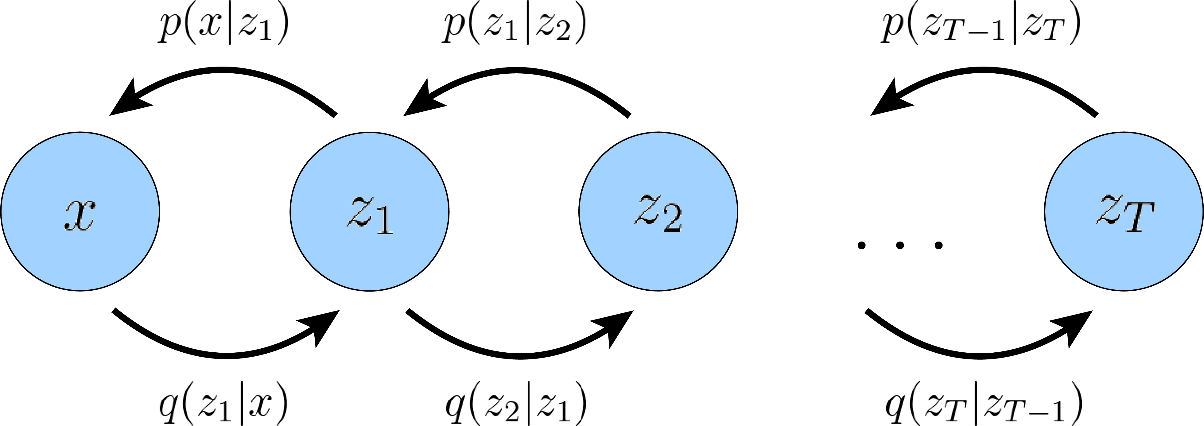
This Markov structure factorises the joint and the posterior into per-step products:

\[ \begin{aligned} p(x, z_{1:T}) &= p(z_T)\, p_\theta(x \mid z_1) \prod_{t=2}^{T} p_\theta(z_{t-1}\mid z_t) \\[4pt] q_\phi(z_{1:T}\mid x) &= q_\phi(z_1 \mid x) \prod_{t=2}^{T} q_\phi(z_t \mid z_{t-1}) \end{aligned} \]

The ELBO extends unchanged, treating \(z_{1:T}\) as a single latent:

\[ \log p(x) = \log \int p(x, z_{1:T})\,\mathrm{d}z_{1:T} \ \ge\ \mathbb{E}_{q_\phi(z_{1:T}\mid x)}\left[\log \frac{p(x, z_{1:T})}{q_\phi(z_{1:T}\mid x)}\right] \]

Substituting the two factorisations turns the bound into a single ratio of products:

\[ \begin{aligned} \mathbb{E}_{q_\phi(z_{1:T}\mid x)}&\left[\log \frac{p(x, z_{1:T})}{q_\phi(z_{1:T}\mid x)}\right] \\[6pt] &= \mathbb{E}_{q_\phi(z_{1:T}\mid x)}\left[\log \frac{p(z_T)\, p_\theta(x\mid z_1) \prod_{t=2}^{T} p_\theta(z_{t-1}\mid z_t)}{q_\phi(z_1\mid x) \prod_{t=2}^{T} q_\phi(z_t \mid z_{t-1})}\right] \\[6pt] &= \mathbb{E}_{q_\phi(z_1\mid x)}\big[\log p_\theta(x\mid z_1)\big] && \text{(reconstruction)} \\[4pt] &\quad + \sum_{t=2}^{T} \mathbb{E}_{q_\phi(z_{t-1}, z_t\mid x)}\left[\log \frac{p_\theta(z_{t-1}\mid z_t)}{q_\phi(z_t\mid z_{t-1})}\right] && \text{(layer-wise transitions)} \\[4pt] &\quad + \mathbb{E}_{q_\phi(z_T\mid x)}\big[\log p(z_T)\big] - \mathbb{E}_{q_\phi(z_1\mid x)}\big[\log q_\phi(z_1\mid x)\big] && \text{(top-level prior, encoder entropy)} \end{aligned} \]

No clean per-step KL yet

\[ \sum_{t=2}^{T} \mathbb{E}_{q_\phi(z_{t-1}, z_t\mid x)}\left[\log \frac{p_\theta(z_{t-1}\mid z_t)}{q_\phi(z_t\mid z_{t-1})}\right] \]

The above term is not a KL divergence, because the two densities are over different variables: \(p_\theta\) is over \(z_{t-1}\) while \(q_\phi\) is over \(z_t\). So the term stays a cross-conditional expectation.

Diffusion models repair it by using Bayes' rule to flip the encoder step into \(q(z_{t-1}\mid z_t, x)\): now both densities are over \(z_{t-1}\), the ratio inverts so that \(q\) sits on the numerator, and the expectation is over the matching distribution. Each step then becomes a genuine, individually computable KL:

\[ -\,\mathbb{E}_{q(z_t\mid x)}\Big[ D_{\text{KL}}\big(q(z_{t-1}\mid z_t, x) \parallel p_\theta(z_{t-1}\mid z_t)\big)\Big] \]

This is the step that makes the VDM objective trainable, and it is the only real gap between the MHVAE bound above and the diffusion ELBO.

Variational Diffusion Models

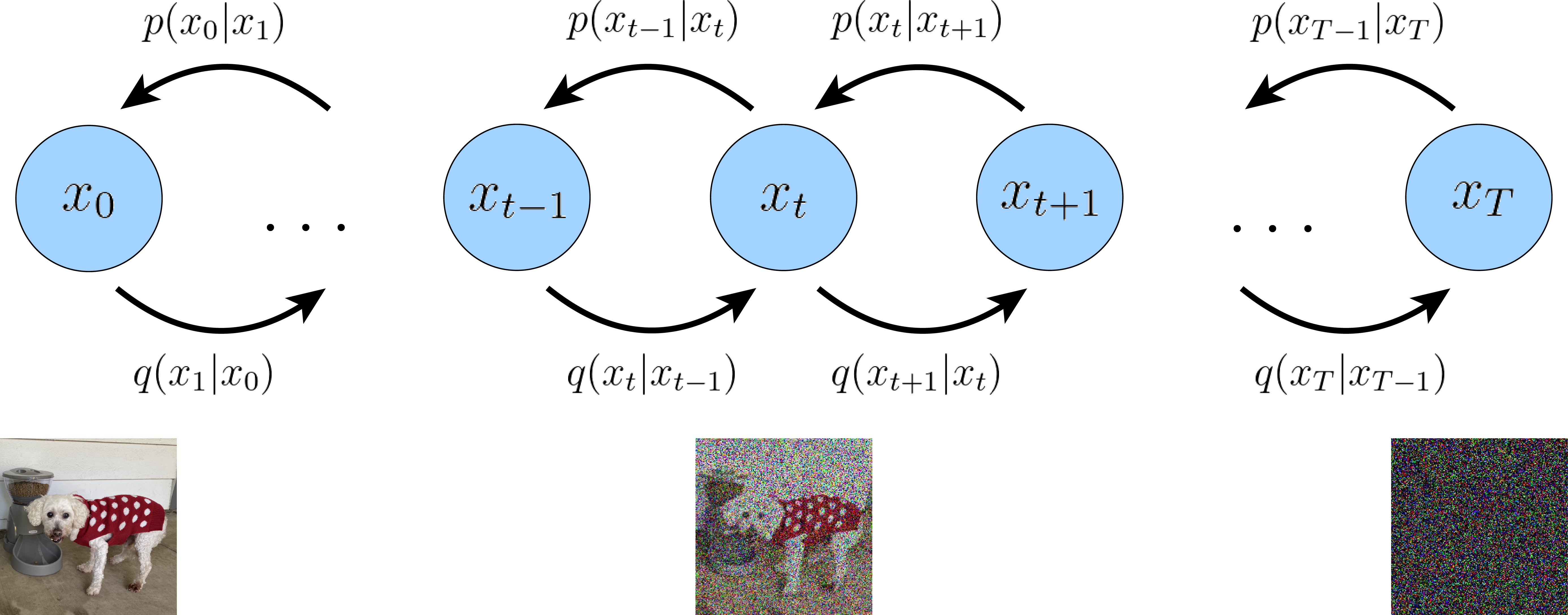
A VDM is an MHVAE with three restrictions:

The latent dimension equals the data dimension — so latents and data share the notation \(x_t\), with \(x_0\) the data and \(t \in [1,T]\) the noise levels.
The encoder is not learned: each step is a fixed linear Gaussian centred on the previous state.
The noise schedule is arranged so that the final latent \(x_T\) is a standard Gaussian.

Variational diffusion model

Forward and reverse process

Forward (noising). The posterior is the same Markov chain as in the MHVAE, now written over \(x_t\):

\[ q(x_{1:T}\mid x_0) = \prod_{t=1}^{T} q(x_t\mid x_{t-1}) \]

Each step is a fixed linear Gaussian centred on the previous state:

\[ q(x_t\mid x_{t-1}) = \mathcal{N}\big(x_t;\, \sqrt{\alpha_t}\,x_{t-1},\, (1-\alpha_t)I\big) \]

The coefficients \(\sqrt{\alpha_t}\) and \(1-\alpha_t\) are chosen so the latents keep a similar scale — the process is variance-preserving. Note there is no \(\phi\): the encoder is a fixed corruption process, not a learned network.

Reverse (denoising). The generative chain runs the other way, starting from pure noise:

\[ p(x_{0:T}) = p(x_T)\prod_{t=1}^{T} p_\theta(x_{t-1}\mid x_t), \qquad p(x_T) = \mathcal{N}(x_T;\, 0, I) \]

Since \(q\) carries no parameters, only the denoising transitions \(p_\theta(x_{t-1}\mid x_t)\) are learned. Sampling means drawing \(x_T \sim \mathcal{N}(0,I)\) and running them \(T\) times.

ELBO: consistency form (Deprecated)

Start from the same Jensen bound as before and substitute the two factorisations, we have:

\[ \begin{aligned} \log p(x) &\ge \mathbb{E}_{q(x_{1:T}\mid x_0)}\left[\log \frac{p(x_{0:T})}{q(x_{1:T}\mid x_0)}\right] && \text{(Jensen)} \\[4pt] &= \mathbb{E}_{q}\left[\log \frac{p(x_T)\prod_{t=1}^{T} p_\theta(x_{t-1}\mid x_t)}{\prod_{t=1}^{T} q(x_t\mid x_{t-1})}\right] && \text{(substitute)} \\[4pt] &= \mathbb{E}_{q}\left[\log \frac{p(x_T)\, p_\theta(x_0\mid x_1) \prod_{t=2}^{T} p_\theta(x_{t-1}\mid x_t)}{q(x_T\mid x_{T-1}) \prod_{t=1}^{T-1} q(x_t\mid x_{t-1})}\right] && \text{(peel off boundaries)} \\[4pt] &= \mathbb{E}_{q}\left[\log \frac{p(x_T)\, p_\theta(x_0\mid x_1) \prod_{t=1}^{T-1} p_\theta(x_t\mid x_{t+1})}{q(x_T\mid x_{T-1}) \prod_{t=1}^{T-1} q(x_t\mid x_{t-1})}\right] && \text{(shift } t \to t+1 \text{ in } p) \\[4pt] &= \mathbb{E}_{q}\big[\log p_\theta(x_0\mid x_1)\big] + \mathbb{E}_{q}\left[\log \frac{p(x_T)}{q(x_T\mid x_{T-1})}\right] + \sum_{t=1}^{T-1}\mathbb{E}_{q}\left[\log \frac{p_\theta(x_t\mid x_{t+1})}{q(x_t\mid x_{t-1})}\right] && \text{(split)} \\[4pt] &= \underbrace{\mathbb{E}_{q(x_1\mid x_0)}\big[\log p_\theta(x_0\mid x_1)\big]}_{\text{reconstruction}} - \underbrace{\mathbb{E}_{q(x_{T-1}\mid x_0)}\big[D_{\text{KL}}(q(x_T\mid x_{T-1}) \parallel p(x_T))\big]}_{\text{prior matching}} \\[4pt] &\quad - \underbrace{\sum_{t=1}^{T-1} \mathbb{E}_{q(x_{t-1},x_{t+1}\mid x_0)}\big[D_{\text{KL}}(q(x_t\mid x_{t-1}) \parallel p_\theta(x_t\mid x_{t+1}))\big]}_{\text{consistency}} && \text{(marginalise, definition of KL)} \end{aligned} \]

Three readings:

Reconstruction — same as the vanilla VAE, predicting \(x_0\) from \(x_1\).
Prior matching — no trainable parameters; for large enough \(T\) the corrupted \(x_T\) is Gaussian and this vanishes.
Consistency — at every intermediate \(x_t\), denoising from above (\(p_\theta(x_t\mid x_{t+1})\)) must match noising from below (\(q(x_t\mid x_{t-1})\)). This dominates the cost, since it runs over all timesteps.

Why this form is not used

The consistency term is an expectation over two random variables \(\{x_{t-1}, x_{t+1}\}\) per timestep. Summed over \(T-1\) steps, its Monte Carlo estimate has high variance.

ELBO: denoising matching form

The fix is to condition on \(x_0\): \(q(x_t\mid x_{t-1}) = q(x_t\mid x_{t-1}, x_0)\) (Markov property) and apply Bayes' rule:

\[ q(x_t \mid x_{t-1}, x_0) = \frac{q(x_{t-1}\mid x_t, x_0)\, q(x_t \mid x_0)}{q(x_{t-1}\mid x_0)} \]

Substituting this into the denominator makes the ratio \(q(x_t\mid x_0)/q(x_{t-1}\mid x_0)\) telescope — consecutive factors cancel, leaving only the two endpoints:

\[ \prod_{t=2}^{T} q(x_t\mid x_{t-1}, x_0) = \prod_{t=2}^{T} q(x_{t-1}\mid x_t, x_0)\cdot \underbrace{\prod_{t=2}^{T}\frac{q(x_t\mid x_0)}{q(x_{t-1}\mid x_0)}}_{=\ q(x_T\mid x_0)\,/\,q(x_1\mid x_0)} \]

Now redo the derivation, this time peeling off only \(t=1\):

\[ \begin{aligned} \log p(x) &\ge \mathbb{E}_{q}\left[\log \frac{p(x_T)\, p_\theta(x_0\mid x_1) \prod_{t=2}^{T} p_\theta(x_{t-1}\mid x_t)}{q(x_1\mid x_0) \prod_{t=2}^{T} q(x_t\mid x_{t-1})}\right] && \text{(peel off } t=1) \\[4pt] &= \mathbb{E}_{q}\left[\log \frac{p(x_T)\, p_\theta(x_0\mid x_1) \prod_{t=2}^{T} p_\theta(x_{t-1}\mid x_t)}{q(x_1\mid x_0) \prod_{t=2}^{T} q(x_t\mid x_{t-1}, x_0)}\right] && \text{(Markov: add } x_0) \\[4pt] &= \mathbb{E}_{q}\left[\log \frac{p(x_T)\, p_\theta(x_0\mid x_1)}{q(x_1\mid x_0)} + \log \frac{q(x_1\mid x_0)}{q(x_T\mid x_0)} + \log \prod_{t=2}^{T}\frac{p_\theta(x_{t-1}\mid x_t)}{q(x_{t-1}\mid x_t, x_0)}\right] && \text{(Bayes + telescope)} \\[4pt] &= \mathbb{E}_{q}\left[\log \frac{p(x_T)\, p_\theta(x_0\mid x_1)}{q(x_T\mid x_0)} + \sum_{t=2}^{T}\log \frac{p_\theta(x_{t-1}\mid x_t)}{q(x_{t-1}\mid x_t, x_0)}\right] && \text{(} q(x_1\mid x_0) \text{ cancels)} \\[4pt] &= \mathbb{E}_{q(x_1\mid x_0)}\big[\log p_\theta(x_0\mid x_1)\big] + \mathbb{E}_{q(x_T\mid x_0)}\left[\log \frac{p(x_T)}{q(x_T\mid x_0)}\right] \\[4pt] &\qquad + \sum_{t=2}^{T} \mathbb{E}_{q(x_t, x_{t-1}\mid x_0)}\left[\log \frac{p_\theta(x_{t-1}\mid x_t)}{q(x_{t-1}\mid x_t, x_0)}\right] && \text{(split, marginalise)} \\[4pt] &= \underbrace{\mathbb{E}_{q(x_1\mid x_0)}\big[\log p_\theta(x_0\mid x_1)\big]}_{\text{reconstruction}} - \underbrace{D_{\text{KL}}\big(q(x_T\mid x_0) \parallel p(x_T)\big)}_{\text{prior matching}} \\[4pt] &\qquad - \sum_{t=2}^{T} \underbrace{\mathbb{E}_{q(x_t\mid x_0)}\big[D_{\text{KL}}\big(q(x_{t-1}\mid x_t, x_0) \parallel p_\theta(x_{t-1}\mid x_t)\big)\big]}_{\text{denoising matching}} && \text{(definition of KL)} \end{aligned} \]

Every term is now an expectation over at most one random variable, which is the whole point: the Monte Carlo estimate has far lower variance than the consistency form. This is the objective actually optimised. The ground-truth denoising step \(q(x_{t-1}\mid x_t, x_0)\) acts as the supervision signal: it says how to denoise \(x_t\) given knowledge of the clean \(x_0\).

Sanity checks

Both derivations use only the Markov assumption, so they hold for any Markovian HVAE. Setting \(T=1\) recovers the vanilla VAE ELBO exactly.

Closed form denoising step

The denoising-matching term needs the ground-truth step \(q(x_{t-1}\mid x_t, x_0)\) in closed form. By Bayes' rule,

\[ q(x_{t-1}\mid x_t, x_0) = \frac{\overbrace{q(x_t\mid x_{t-1}, x_0)}^{\text{known}}\,\overbrace{q(x_{t-1}\mid x_0)}^{?}}{\underbrace{q(x_t\mid x_0)}_{?}} \]

The forward step \(q(x_t\mid x_{t-1}, x_0) = q(x_t\mid x_{t-1}) = \mathcal{N}(x_t;\sqrt{\alpha_t}\,x_{t-1},(1-\alpha_t)I)\) is already given. What we still need is the marginal \(q(x_t\mid x_0)\) — how noise accumulates from the clean image directly to step \(t\).

Three Gaussian algebra rules

For independent \(X_1\sim\mathcal{N}(\mu_1,\sigma_1^2)\) and \(X_2\sim\mathcal{N}(\mu_2,\sigma_2^2)\):

Scaling: \(aX_1 \sim \mathcal{N}(a\mu_1,\, a^2\sigma_1^2)\) — mean scales by \(a\), variance by \(a^2\) (so the std scales by \(|a|\)).
Sum: \(X_1 + X_2 \sim \mathcal{N}(\mu_1+\mu_2,\, \sigma_1^2+\sigma_2^2)\) — means add, variances add (not stds).
Merging two noises ("Pythagoras"): combining the above for \(\epsilon_1,\epsilon_2\sim\mathcal{N}(0,I)\),

\[ a\,\epsilon_1 + b\,\epsilon_2 = \sqrt{a^2+b^2}\,\epsilon, \qquad \epsilon\sim\mathcal{N}(0,I) \]

Think of \(a,b\) as the legs of a right triangle and the merged amplitude as the hypotenuse \(\sqrt{a^2+b^2}\). This is exactly the cancellation below: \(\big(\sqrt{\alpha_t}\sqrt{1-\alpha_{t-1}}\big)^2 + \big(\sqrt{1-\alpha_t}\big)^2 = \alpha_t - \alpha_t\alpha_{t-1} + 1-\alpha_t = 1-\alpha_t\alpha_{t-1}\).

Deriving \(q(x_t\mid x_0)\). Unroll the forward recursion with the reparameterisation trick, repeatedly merging two independent Gaussian noises into one (means add, variances add). With \(\bar\alpha_t = \prod_{i=1}^{t}\alpha_i\):

\[ \begin{aligned} x_t &= \sqrt{\alpha_t}\,x_{t-1} + \sqrt{1-\alpha_t}\,\epsilon_{t-1}^* \\[4pt] &= \sqrt{\alpha_t}\big(\sqrt{\alpha_{t-1}}\,x_{t-2} + \sqrt{1-\alpha_{t-1}}\,\epsilon_{t-2}^*\big) + \sqrt{1-\alpha_t}\,\epsilon_{t-1}^* \\[4pt] &= \sqrt{\alpha_t\alpha_{t-1}}\,x_{t-2} + \sqrt{1-\alpha_t\alpha_{t-1}}\,\epsilon_{t-2} && \text{(merge the two noises)} \\[4pt] &\ \ \vdots \\[4pt] &= \sqrt{\textstyle\prod_{i=1}^{t}\alpha_i}\,x_0 + \sqrt{1-\textstyle\prod_{i=1}^{t}\alpha_i}\,\epsilon_0 = \sqrt{\bar\alpha_t}\,x_0 + \sqrt{1-\bar\alpha_t}\,\epsilon_0 \end{aligned} \]

so that

\[ q(x_t\mid x_0) = \mathcal{N}\big(x_t;\, \sqrt{\bar\alpha_t}\,x_0,\, (1-\bar\alpha_t)I\big) \]

Assembling the posterior. All three factors are now Gaussian. Substituting into Bayes' rule and completing the square in \(x_{t-1}\) gives

\[ q(x_{t-1}\mid x_t, x_0) = \mathcal{N}\big(x_{t-1};\, \mu_q(x_t, x_0),\, \Sigma_q(t)\big), \qquad \mu_q(x_t, x_0) = \frac{\sqrt{\alpha_t}(1-\bar\alpha_{t-1})x_t + \sqrt{\bar\alpha_{t-1}}(1-\alpha_t)x_0}{1-\bar\alpha_t} \]

with \(\Sigma_q(t) = \sigma_q^2(t)I\) and \(\sigma_q^2(t) = \dfrac{(1-\alpha_t)(1-\bar\alpha_{t-1})}{1-\bar\alpha_t}\). Both depend only on the fixed \(\alpha\) schedule, so this posterior is fully known — the perfect regression target for \(p_\theta\).

Completing the square = matching two coefficients

A Gaussian is determined by only two numbers, so its exponent — a quadratic in \(x_{t-1}\) — carries only two pieces of information. Expanding the target form makes them explicit:

\[ -\frac{(x_{t-1}-\mu_q)^2}{2\sigma_q^2} = -\frac{1}{2}\left[\frac{1}{\sigma_q^2}\,x_{t-1}^2 - 2\,\frac{\mu_q}{\sigma_q^2}\,x_{t-1} + C\right] \]

So the entire derivation is: whatever multiplies \(x_{t-1}^2\) is \(\tfrac{1}{\sigma_q^2}\), and whatever multiplies \(x_{t-1}\) is \(-2\tfrac{\mu_q}{\sigma_q^2}\) — everything without an \(x_{t-1}\) is an irrelevant constant. Expanding the numerator \(q(x_t\mid x_{t-1})\,q(x_{t-1}\mid x_0)\) and collecting these two:

\[ \frac{1}{\sigma_q^2} = \frac{\alpha_t}{1-\alpha_t} + \frac{1}{1-\bar\alpha_{t-1}} = \frac{1-\bar\alpha_t}{(1-\alpha_t)(1-\bar\alpha_{t-1})}, \qquad \frac{\mu_q}{\sigma_q^2} = \frac{\sqrt{\alpha_t}\,x_t}{1-\alpha_t} + \frac{\sqrt{\bar\alpha_{t-1}}\,x_0}{1-\bar\alpha_{t-1}} \]

(the first uses \(\alpha_t\bar\alpha_{t-1} = \bar\alpha_t\)). Now \(\sigma_q^2\) is just the reciprocal of the first, and \(\mu_q = \sigma_q^2 \cdot (\text{second})\) — the shared denominator \((1-\alpha_t)(1-\bar\alpha_{t-1})\) cancels, giving the clean forms above.

From KL to a regression loss

Model \(p_\theta(x_{t-1}\mid x_t)\) as a Gaussian with the same variance \(\Sigma_q(t)\) — legitimate since all \(\alpha\) are fixed. The KL between two Gaussians of equal covariance reduces to a distance between means:

\[ \arg\min_\theta D_{\text{KL}}\big(q(x_{t-1}\mid x_t,x_0) \parallel p_\theta(x_{t-1}\mid x_t)\big) = \arg\min_\theta \frac{1}{2\sigma_q^2(t)}\left\lVert \mu_\theta(x_t, t) - \mu_q(x_t, x_0) \right\rVert_2^2 \]

Since \(\mu_\theta\) may not condition on \(x_0\), match \(\mu_q\) by substituting a network prediction \(\hat{x}_\theta(x_t, t)\) in place of \(x_0\). Everything else cancels:

\[ \arg\min_\theta D_{\text{KL}}(\cdot \parallel \cdot) = \arg\min_\theta \frac{1}{2\sigma_q^2(t)}\frac{\bar\alpha_{t-1}(1-\alpha_t)^2}{(1-\bar\alpha_t)^2} \left\lVert \hat{x}_\theta(x_t, t) - x_0 \right\rVert_2^2 \]

So training a VDM reduces to a neural network predicting the clean image from a noisy one. In practice the sum over \(t\) is replaced by a uniform sample:

\[ \arg\min_\theta\ \mathbb{E}_{t\sim U\{2,T\}}\Big[\mathbb{E}_{q(x_t\mid x_0)}\big[D_{\text{KL}}\big(q(x_{t-1}\mid x_t,x_0)\parallel p_\theta(x_{t-1}\mid x_t)\big)\big]\Big] \]